


| Plotting graphs | |
| plot | graph an expression of one variable |
| plotfunc | graph an expression of one or two variables |
| tangent | tangent to a curve |
| plotparam | parametric curve |
| plotpolar | polar plotting |
| plotimplicit | implicit curve |
The Graphic menu has entries for several graphing commands; if you choose one you will be given a template you can fill out to produce a graphic. The appropriate command will be placed on the command line. If you want several graphs in the same window, you can put the commands on the same command line separated by semicolons.
Once you have created a graphic window, there will be a panel to the right with buttons allowing you to control the image. The default parameters for graphs, such as the size of the graphs, are configurable (see section 2.3, “Configuration”).
As well as being displayed in the Xcas window, the two dimensional graphics also appear in the DispG (Display Graphics) window. You can bring that window up with the Cfg▸Show▸DispG menu item. This window will contain all two dimensional graphs; they can be cleared with the ClrGraph command.
The simplest way to draw graphs is with the templates from the Graphic menu, but there are command line equivalents.
The command line instruction for graphing a function is the plot command. It takes an expression (or list of expressions) followed by the variable. To use a domain different than the default, you can indicate the range of the variable by setting it equal to an interval. If you are plotting several curves, you can distinguish them by giving them different colors; you can do this with a third argument color= followed by a list of colors. If you plot
plot([x^2,x^3],x=-1..1,color=[red,blue])
you will get

You can draw parameterized curves with the plotparam command. The coordinates of the curve must be given as a single complex expression; the x coordinate will be the real part of the expression and the y coordinate will be the imaginary part. For example, if you enter
plotparam(sin(t) + i*cos(t),t)
you will get the circle

(Since the x- and y-axes are scaled differently, the circle looks elliptical.)
You can draw a curve using polar coordinates with the plotpolar command. This takes the form plotpolar(f(theta),theta,theta-min,theta-max).
You can draw an implicitly defined curve with the plotimplicit command; the command plotimplicit(f(x,y),x,y) will draw the curve f(x,y)=0. For example, the command
plotimplicit(x^2 + y^2 = 1,x,y)
will draw a circle.
The tangent command will draw the tangent line to a curve, if you tell it the curve and the point. To draw the tangent line to the graph y=x2 at x=1, for example, you can enter
tangent(plotfunc(x^2,x),1)
You will get

| 2D graphical objects | |
| legend | place text starting from a given point |
| point | determine a point given a complex number or two coordinates |
| segment | segment determined by 2 points |
| circle | circle determined by a point and radius |
| inter | find the intersection of curves |
| equation | return the cartesian equation of a curve |
| parameq | return the parametric equation of a curve |
| polygonplot | draw a polygonal line |
| scatterplot | draw a cloud of dots |
| polygon | draw a closed polygon |
| open_polygon | draw an open polygon |
Among its other capabilities, Xcas works with plane geometry. The Geo▸New figure 2D menu item or the Alt+g key will bring up the screen for plane geometry.
A point on the geometry screen can be specified with the point command, which can take either an ordered pair or real numbers or a complex number as argument. The Geo menu contains many commands for drawing geometric objects, such as circle (which takes a point and a radius as arguments) and polygon (which takes a sequence of points as arguments).
Some functions, such as polygonplot and scatterplot, take lists of x-coordinates and y-coordinates as arguments. For example,
polygonplot([0,2,0],[0,0,2])
and
open_polygon(point(0,0),point(2,0),point(0,2))
will both draw the same segments.
The legend can be used to place text on the screen; one simple way of using it is to give it a point and text as arguments.
| 3D graphical objects | |
| plotfunc | graph of a function |
| plotparam | parametric surface |
| point | point |
| plane | plane |
| sphere | sphere with a center and radius |
| cone | cone with a center, axis and opening angle |
| inter | intersection |
| polygon | polygon |
| open_polygon | open polygon |
Xcas can also handle three-dimensions graphically, either by drawing curves and graphs in three-dimensions or by drawing three-dimensional geometric objects. A three-dimensional screen can be brought up with the Geo▸New figure 3D menu item or the Alt+h key. There will controls for the view window to the right of the screen. You can rotate the visualization cube by using the mouse outside of the cube or by clicking in the cube and using the x, y and z keys to rotate and the + and - keys for zooming.
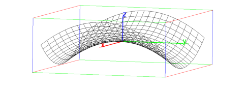
You can draw a graph z = f(x,y) with the plotfunc command, which takes an expression and a list of two variables. Like graphs of functions of one variable, you can use a domain different than the default by giving the variables their own intervals. The command
plotfunc(y^2 - x^2,[x=-1..1,y=-1..1])
will give you the graph
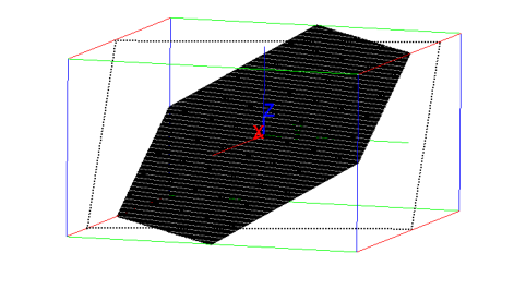
The plotparam command can be used to draw a parameterized curves and surfaces in three-dimensions. If the first argument is a list of three expressions involving two variables and the next two arguments are the variables (with optional intervals), then plotparam will plot the surface. If you enter
plotparam([u,u+v,v],u,v)
you will get
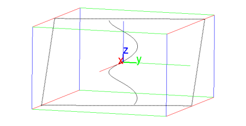
If the first argument is a list of three expressions involving one variable and the next argument is the variable, then plotparam will plot the curve. If you enter
plotparam([cos(t),sin(t),t],t)
you will get
A point in three-dimensions is given with the point command with three arguments. Commands like polygon and open_polygon work in three-dimensions as well as two, as well as additional commands such as sphere. A plane can be drawn with the plane command, which can be given either three points, a line and two points, or an equation of the form a*x + b*y + c*z = d.